De-Noising Quasar Spectra
- 9 mins
A quasar can be defined as an extremely Active Galactic Nucleus (AGN). An AGN is nothing more than a supermassive black hole that is active and feeding at the center of a galaxy. They are extremely bright and sometimes mistaken for stars. However, the energy output of a star is nowhere near the amount of energy pumped out by a quasar. The word “quasar” originates from the contraction of “quasi-stellar”, which references a star-like radio source.
Properties of Quasars :
The electromagnetic spectrum gives us the range of frequencies of different electromagnetic waves and their respective wavelengths. There are different electromagnetic wave regions, based on their frequency.
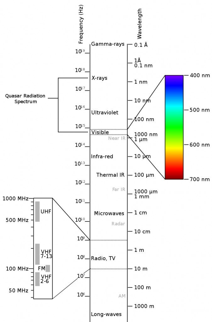
Quasars are known to emit electromagnetic radiation, which lies between the visible and X-ray regions. They also emit large amounts of ultraviolet waves.
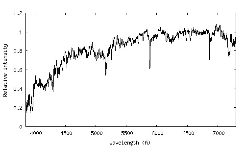
Quasar Spectra for “Messier 31” Galaxy is shown below :
Understanding the properties of the spectrum of the light emitted by a quasar is useful for a number of tasks :
- A number of quasar properties can be estimated from the spectra.
- Properties of the regions of the universe through which the light passes can also be evaluated. For example, in estimating the density of neutral and ionized particles in the universe, which helps cosmologists understand the evolution and fundamental laws governing its structure.
The light spectrum is a curve that relates the light’s intensity (formally, lumens per square meter), or luminous flux, to its wavelength. The wavelengths are measured in Angstroms (°A), where 1°A= 10^(−10) meters.
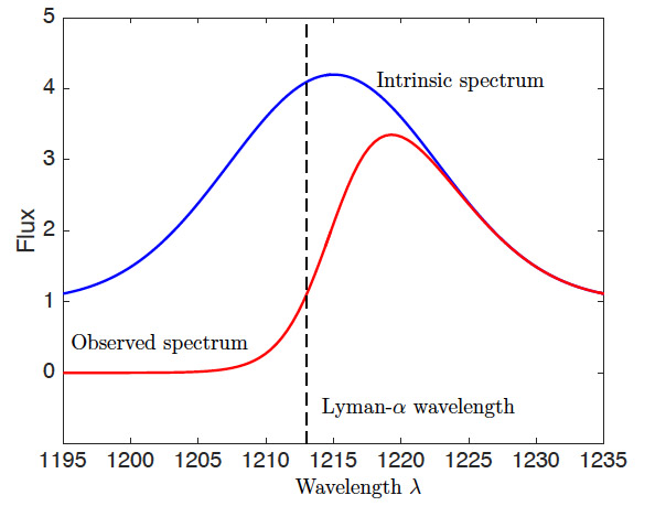
The blue line shows the intrinsic (i.e. original) flux spectrum emitted by the quasar. The red line denotes the observed spectrum here on Earth. To the left of the Lyman- α line, the observed flux is damped and the intrinsic (unabsorbed) flux continuum is not clearly recognizable (red line). To the right of the Lyman-α line, the observed flux approximates the intrinsic spectrum.
The Lyman-α wavelength is a wavelength beyond which intervening particles at most negligibly interfere with light emitted from the quasar. (Interference generally occurs when a photon is absorbed by a neutral hydrogen atom, which only occurs for certain wavelengths of light.) For wavelengths greater than this Lyman-α wavelength, the observed light spectrum f_obs can be modeled as a smooth spectrum f plus noise:
For wavelengths below the Lyman-α wavelength, a region of the spectrum known as the Lyman-α forest, intervening matter causes attenuation of the observed signal. As light emitted by the quasar travels through regions of the universe richer in neutral hydrogen, some of it is absorbed, which modeled as
Astrophysicists and cosmologists wish to understand the absorption function, which gives infor- mation about the Lyman-α forest, and hence the distribution of neutral hydrogen in otherwise unreachable regions of the universe. This gives clues toward the formation and evolution of the universe. Thus, it is our goal to estimate the spectrum f of an observed quasar.
Getting the data :
Used data generated from the Hubble Space Telescope Faint Object Spectrograph (HST-FOS), Spectra of Active Galactic Nuclei and Quasars. Dataset
I wish to predict an entire part of a spectrum—a curve—from noisy observed data. I begin by supposing that I observe a random sample of m absorption-free spectra, which is possible for quasars very close (in a sense relative to the size of the universe!) to Earth. For a given spectrum f, define f_right to be the spectrum to the right of the Lyman-α line. Let f_left be the spectrum within the Lyman-α forest region, that is, for lower wavelengths. To make the results cleaner, defined as:
wl_right = wave_lens[wave_lens >= 1300]
wl_left = wave_lens[wave_lens < 1200]
Will learn a function r (for regression) that maps an observed f_right to an unobserved target f_left (note that f_left and f_right don’t cover the entire spectrum). This is useful in practice because I observe f_right with only random noise: there is no systematic absorp- tion, which I cannot observe directly, because hydrogen does not absorb photons with higher wavelengths. By predicting f_left from a noisy version of f_right, Now I can estimate the unobservable spectrum of a quasar as well as the absorption function. Imaging systems collect data of the form
for λ ∈ {λ1, . . . , λn}, a finite number of points λ, because they must quantize the information. That is, even in the quasars-close-to-Earth training data, our observations of f_left and f_right consist of noisy evaluations of the true spectrum f at multiple wavelengths. In this case,I have n = 450 and λ1 = 1150, . . . , λn = 1599.
Formulate the functional regression task as the goal of learning the function r mapping f_right to f_left:
To estimate the unobserved spectrum f_left of a quasar from its (noisy) observed spectrum f_right. To do so, I perform a weighted regression of the locally weighted regressions. In particular, given a new noisy spectrum observation:
for λ ∈ {1300, . . . , 1599}.
I define a metric d which takes as input, two spectra f1 and f2, and outputs a scalar:
That is in python :
dists = ((df_fs_test_r - row) ** 2).sum(axis=1)
The metric d computes squared distance between the new datapoint and previous datapoints. If f1 and f2 are right spectra, then I take the preceding sum only over λ ∈ {1300, . . . , 1599}, rather than the entire spectrum.
Based on this distance function, I may define the nonparametric functional regression estimator, which is a locally weighted sum of functions f_left from the training data (this is like locally weighted linear regression, except that instead of predicting y ∈ R , predict a function f_left). Specifically, let f_right denote the right side of a spectrum, which I have smoothed using locally weighted linear regression. I wish to estimate the associated left spectrum f_left. Define the function ker(t) = max{1 − t, 0} and let neighb_k(f_right) denote the k indices i ∈ {1, 2, . . . ,m} of the training set that are closest to f_right.
# It's very similar to k-nearest-neighbour algorithm,
# it select the neihbours based on distances calculated from the right spectrum

num_neighb = 3 # number of neighbours to consider
errors = []
preds_tv = []

for k, row in df_fs_tv_r.iterrows():
    dists = ((df_fs_tv_r - row) ** 2).sum(axis=1)
    max_d = dists.max()
    neighb_ds = dists.sort_values()[:num_neighb]

    p1 = np.sum([ker(d / max_d) * df_fs_tv_l.loc[idx] for (idx, d) in neighb_ds.iteritems()], axis = 0)
    p2 = np.sum([ker(d / max_d) for (idx, d) in neighb_ds.iteritems()])

    f_left_hat = p1/p2
    preds_tv.append(f_left_hat)
    error = np.sum((f_left_hat - df_fs_tv_l.loc[k])**2)
    errors.append(error)
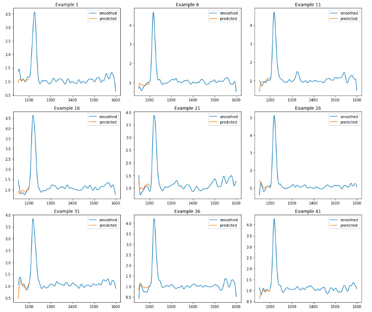
I also visualized some of the predictions on the train dataset:
fig, axes = plt.subplots(3,3,figsize=(14,12))
axes = axes.ravel()

for k, idx in enumerate([0,5,10,15,20,25,30,35,40]):
    ax = axes[k]
    ax.plot(wave_lens, df_fs_tv.loc[idx], label='smoothed')
    ax.plot(wl_left, preds_tv[idx], label='predicted')
    ax.legend()
    ax.set_title("Example {0}".format(idx + 1))

plt.tight_layout()
After working on the training dataset, finally I moved to the test datadset and predicted the quasar spectrum. To view the Python Notebook click here.
Prediction on test data :
fig, axes = plt.subplots(3, 3, figsize=(14, 12))
axes = axes.ravel()
for k, idx in enumerate([3, 7, 13, 17, 22, 28, 33, 36, 40]):
    ax = axes[k]
    ax.plot(wave_lens, df_fs_test.loc[idx], label='smoothed')
    ax.plot(wl_left, preds_test[idx], label='predicted')
    ax.legend()
    ax.set_title('Example {0}'.format(idx + 1))
plt.tight_layout()
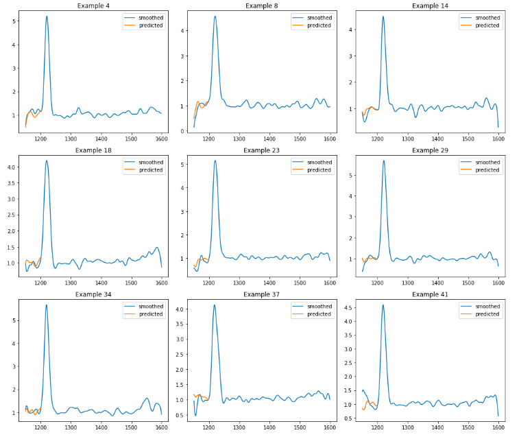
Overall, the prediction was not as good as it was expected, for both training and testing data.
References :
- Ciollaro, Mattia, et al. “Functional regression for quasar spectra.” arXiv:1404.3168 (2014)
- https://www.scienceabc.com/pure-sciences/what-are-quasars.html
- http://www.astrosurf.com/buil/galaxies/spectra.html